Tissue classification from MP2RAGE data

This example shows how to obtain a tissue classification from MP2RAGE data by performing the following steps:

1. Downloading open MP2RAGE dataset using nighres.data.download_7T_TRT()
2. Remove the skull and create a brain mask using nighres.brain.mp2rage_skullstripping()
3. Atlas-guided tissue classification using MGDM nighres.brain.mgdm_segmentation() [1]

Import and download

First we import nighres and the os module to set the output directory Make sure to run this file in a directory you have write access to, or change the out_dir variable below.

import nighres
import os

in_dir = os.path.join(os.getcwd(), 'nighres_examples/data_sets')
out_dir = os.path.join(os.getcwd(), 'nighres_examples/tissue_classification')

We also try to import Nilearn plotting functions. If Nilearn is not installed, plotting will be skipped.

skip_plots = False
try:
    from nilearn import plotting
except ImportError:
    skip_plots = True
    print('Nilearn could not be imported, plotting will be skipped')

Now we download an example MP2RAGE dataset. It is the structural scan of the first subject, first session of the 7T Test-Retest dataset published by Gorgolewski et al (2015) [2].

dataset = nighres.data.download_7T_TRT(in_dir, subject_id='sub001_sess1')

Skull stripping

First we perform skull stripping. Only the second inversion image is required to calculate the brain mask. But if we input the T1map and T1w image as well, they will be masked for us. We also save the outputs in the out_dir specified above and use a subject ID as the base file_name.

skullstripping_results = nighres.brain.mp2rage_skullstripping(
                                            second_inversion=dataset['inv2'],
                                            t1_weighted=dataset['t1w'],
                                            t1_map=dataset['t1map'],
                                            save_data=True,
                                            file_name='sub001_sess1',
                                            output_dir=out_dir)

Tip

in Nighres functions that have several outputs return a dictionary storing the different outputs. You can find the keys in the docstring by typing nighres.brain.mp2rage_skullstripping? or list them with skullstripping_results.keys()

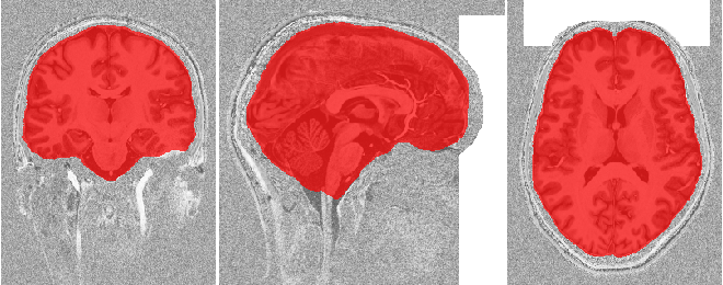
To check if the skull stripping worked well we plot the brain mask on top of the original image. You can also open the images stored in out_dir in your favourite interactive viewer and scroll through the volume.

Like Nilearn, we use Nibabel SpatialImage objects to pass data internally. Therefore, we can directly plot the outputs using Nilearn plotting functions .

if not skip_plots:
    plotting.plot_roi(skullstripping_results['brain_mask'], dataset['t1w'],
                      annotate=False, black_bg=False, draw_cross=False,
                      cmap='autumn')

MGDM classification

Next, we use the masked data as input for tissue classification with the MGDM algorithm. MGDM works with a single contrast, but can be improved with additional contrasts. In this case we use the T1-weigthed image as well as the quantitative T1map.

mgdm_results = nighres.brain.mgdm_segmentation(
                        contrast_image1=skullstripping_results['t1w_masked'],
                        contrast_type1="Mp2rage7T",
                        contrast_image2=skullstripping_results['t1map_masked'],
                        contrast_type2="T1map7T",
                        save_data=True, file_name="sub001_sess1",
                        output_dir=out_dir)

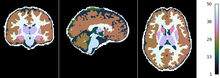
Now we look at the topology-constrained segmentation MGDM created

if not skip_plots:
    plotting.plot_img(mgdm_results['segmentation'],
                      vmin=1, vmax=50, cmap='cubehelix',  colorbar=True,
                      annotate=False,  draw_cross=False)

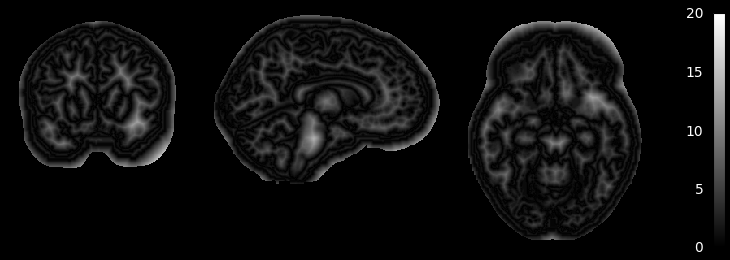
MGDM also creates an image which represents for each voxel the distance to its nearest border. It is useful to assess where partial volume effects may occur

if not skip_plots:
    plotting.plot_anat(mgdm_results['distance'], vmin=0, vmax=20,
                       annotate=False, draw_cross=False, colorbar=True)

If the example is not run in a jupyter notebook, render the plots:

if not skip_plots:
    plotting.show()

References

[1]	Bogovic, Prince and Bazin (2013). A multiple object geometric deformable model for image segmentation. DOI: 10.1016/j.cviu.2012.10.006.A

[2]	Gorgolewski et al (2015). A high resolution 7-Tesla resting-state fMRI test-retest dataset with cognitive and physiological measures. DOI: 10.1038/sdata.2014.54