DOTS white matter segmentation

This example shows how to perform white matter segmentation using Diffusion Oriented Tract Segmentation (DOTS) algorithm [1]:

1. Downloading DOTS atlas prior informationg using

   nighres.data.download_DOTS_atlas()

2. Downloading an example DTI data set using

   nighres.data.download_DTI_2mm()

3. Segmenting white matter in DTI images into major tracts using

   nighres.brain.dots_segmentation()

4. Visualizing the results using matplotlib

Import and download

First we import nighres and os to set the output directory. Make sure to run this file in a directory you have write access to, or change the out_dir variable below. We can downloadthe DOTS atlas priors and an example DTI dataset using the following command. The registration step of the DOTS function relies on dipy, so make sure you have installed it (https://nipy.org/dipy/).

import os
import dipy
import nighres

in_dir = os.path.join(os.getcwd(), 'nighres_examples/data_sets')
out_dir = os.path.join(os.getcwd(), 'nighres_examples/dots_segmentation')
atlas_dir = os.path.join(os.getcwd(), 'nighres_examples')
nighres.data.download_DOTS_atlas(atlas_dir)
dataset = nighres.data.download_DTI_2mm(in_dir)

We also try to import Nilearn plotting functions. If Nilearn is not installed, plotting will be skipped.

skip_plots = False
try:
    from nilearn import plotting
except ImportError:
    skip_plots = True
    print('Nilearn could not be imported, plotting will be skipped')

White matter segmentation

The DOTS segmentation can be run as follows. By default, the algorithm uses the tract atlas consisting of 23 tracts specified in [2]. This can be changed to the full atlas by changing the value of the parameter ‘wm_atlas’ to 2. Please see documentation for details.

dots_results = nighres.brain.dots_segmentation(tensor_image=dataset['dti'],
                                               mask=dataset['mask'],
                                               atlas_dir=atlas_dir,
                                               save_data=True,
                                               output_dir=out_dir,
                                               file_name='example')

segmentation = nighres.io.load_volume(dots_results['segmentation']).get_data()
posterior = nighres.io.load_volume(dots_results['posterior']).get_data()

Tip

The parameter values of the DOTS algorithm can have a significant effect on segmentation results. Experiment with changing their values to obtain optimal results.

Interpretation of results

The integers in the segmentation array and the fourth dimension of the posterior array correspond to the tracts specified in atlas_labels_1 (in case of using wm_atlas 1) which can be imported as follows

from nighres.brain.dots_segmentation import atlas_labels_1

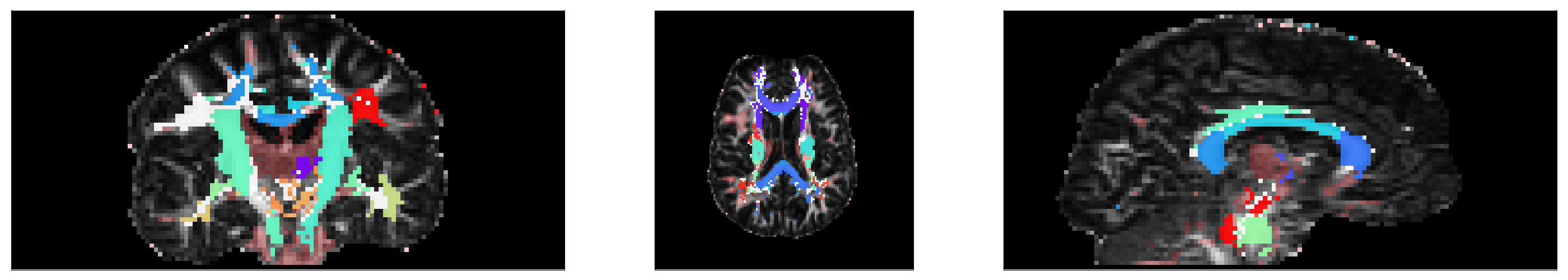
Visualization of results

We can visualize the segmented tracts overlaid on top of a fractional anisotropy map. Let’s first import the necessary modules and define a colormap. Then, we calculate the FA map and show the tracts. Let’s also show the posterior probability distribution of an individual tract.

import numpy as np
import nibabel as nb
import matplotlib.pyplot as plt
from matplotlib import cm
from matplotlib.colors import ListedColormap

# This defines the following colormap
# transparent = isotropic
# semi-transparent red = unclassified white matter
# opaque colours = individual tracts
# white = overlapping tracts

N_t = 23 # 41 if using atlas 2
N_o = 50 # 185 is using atlas 2
newcolors = np.zeros((N_t + N_o, 4))
newcolors[0,:] = np.array([.2, .2, .2, 0])
newcolors[1,:] = np.array([1, 0, 0, .25])
rainbow = cm.get_cmap('rainbow', N_t - 2)
newcolors[2:N_t,:] = rainbow(np.linspace(0, 1, N_t - 2))
newcolors[N_t::,:] = np.ones(newcolors[N_t::,:].shape)
newcmp = ListedColormap(newcolors)

# Calculate FA
tensor_img = nb.load(os.path.join(in_dir, 'DTI_2mm/DTI_2mm.nii.gz'))
tensor_volume = tensor_img.get_data()
xs, ys, zs, _ = tensor_volume.shape
tenfit = np.zeros((xs, ys, zs, 3, 3))
tenfit[:,:,:,0,0] = tensor_volume[:,:,:,0]
tenfit[:,:,:,1,1] = tensor_volume[:,:,:,1]
tenfit[:,:,:,2,2] = tensor_volume[:,:,:,2]
tenfit[:,:,:,0,1] = tensor_volume[:,:,:,3]
tenfit[:,:,:,1,0] = tensor_volume[:,:,:,3]
tenfit[:,:,:,0,2] = tensor_volume[:,:,:,4]
tenfit[:,:,:,2,0] = tensor_volume[:,:,:,4]
tenfit[:,:,:,1,2] = tensor_volume[:,:,:,5]
tenfit[:,:,:,2,1] = tensor_volume[:,:,:,5]
tenfit[np.isnan(tenfit)] = 0
evals, evecs = np.linalg.eig(tenfit)
R = tenfit / np.trace(tenfit, axis1=3, axis2=4)[:,:,:,np.newaxis,np.newaxis]
FA = np.sqrt(0.5 * (3 - 1/(np.trace(np.matmul(R,R), axis1=3, axis2=4))))
FA[np.isnan(FA)] = 0
# save for convenience
nighres.io.save_volume(os.path.join(out_dir, 'FA.nii.gz'),
    nb.Nifti1Image(FA,tensor_img.affine,tensor_img.header))

# Show segmentation
fig, ax = plt.subplots(1, 3, figsize=(28,5))
ax[0].imshow(np.rot90(FA[:,60,:]), cmap = 'gray', vmin = 0, vmax = 1)
ax[0].imshow(np.rot90(segmentation[:,60,:]), cmap=newcmp, alpha=.9)
ax[1].imshow(np.rot90(FA[:,:,30]), cmap = 'gray', vmin = 0, vmax = 1)
ax[1].imshow(np.rot90(segmentation[:,:,30]), cmap=newcmp, alpha=.9)
ax[2].imshow(np.rot90(FA[60,:,:]), cmap = 'gray', vmin = 0, vmax = 1)
ax[2].imshow(np.rot90(segmentation[60,:,:]), cmap=newcmp, alpha=.9)
for i in range(3):
    ax[i].set_xticks([])
    ax[i].set_yticks([])
fig.tight_layout()
#fig.savefig('segmentation.png')
plt.show()

# Show posterior probability of the left corticospinal tract
tract_idx = 9
fig, ax = plt.subplots(1, 3, figsize=(28,5))
ax[0].imshow(np.rot90(FA[:,60,:]), cmap = 'gray', vmin = 0, vmax = 1)
ax[0].imshow(np.rot90(posterior[:,60,:,tract_idx]), alpha = .75)
ax[1].imshow(np.rot90(FA[:,:,30]), cmap = 'gray', vmin = 0, vmax = 1)
ax[1].imshow(np.rot90(posterior[:,:,30,tract_idx]), alpha=.75)
ax[2].imshow(np.rot90(FA[75,:,:]), cmap = 'gray', vmin = 0, vmax = 1)
ax[2].imshow(np.rot90(posterior[75,:,:,tract_idx]), alpha=.75)
for i in range(3):
    ax[i].set_xticks([])
    ax[i].set_yticks([])
fig.tight_layout()
#fig.savefig('CST_posterior.png')
plt.show()

References

[1]	Bazin, Pierre-Louis, et al. “Direct segmentation of the major white matter tracts in diffusion tensor images.” Neuroimage (2011) doi: https://doi.org/10.1016/j.neuroimage.2011.06.020

[2]	Bazin, Pierre-Louis, et al. “Efficient MRF segmentation of DTI white matter tracts using an overlapping fiber model.” Proceedings of the International Workshop on Diffusion Modelling and Fiber Cup (2009)